Pulse decoders [Advanced Radio Control (1965)]

There are limitations as to the number of tone channels that can be operated simultaneously on a single rf carrier. There are other methods which will permit the number of possible channels to be increased.

For example, it is possible to use subcarriers-a method similar to that used for FM stereo broadcasting.

The subcarrier of, say, 100 khz is modulated with perhaps six tones.

A second subcarrier of, say, 150 khz is modulated with another six tones. The radio control transmitter carrier then is modulated with these two subcarriers. In the receiving equipment, bandpass filters first separate the subcarriers, and then additional bandpass filters extract each of the six tones from each subcarrier.

This method, of course, increases the number of tone channels which can be transmitted for simultaneous and proportional control.

Subcarriers of 10, 15 and 20 khz can be used, provided the tones are in still lower frequencies of 100 to 600 cycles per second.

The use of pulses will probably give the greatest flexibility and versatility in control signal applications. These pulses can be either tone or carrier types. We will consider that the normal uses such as pulse-width--pulse-spacing variations are already well known.

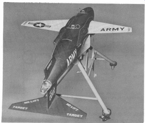
Fig. 401. Drone aircraft can be radio-controlled.

There are many possibilities for using high speed pulses and electronic decoding methods to obtain simultaneous and proportional control over many functions. Note that when we speak of high speed pulses we mean that pulses will be sent so fast, with respect to the equipment operation, that even though they actually are not trans mitted simultaneously, as far as our equipment is concerned they will seem to be received simultaneously. The rate of pulse transmission will be determined by the equipment to be controlled. Fig. 401 shows a drone aircraft which could be controlled by pulse transmission. The reduced wing span and tail design is for high speed flying.

The basic circuits

Some of the basic circuits which are used in pulse control applications are the monostable and the bistable multivibrators.

Figs. 402-a and 402-b are schematics of two types of monostable multivibrators. In Fig. 402-a, there are two possible outputs, e01 and e02. Note that the emitters are connected together and have a common emitter resistor. In this circuit, Q2 is normally conducting at its ...

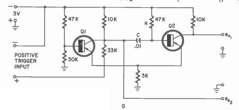
Fig. 402-a. Two-transistor mono-stable multivibrator with two outputs.

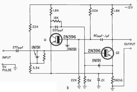
Fig. 402-b. Monostable multi-vibrator, one output.

... saturation value and Q1 is cut off. When a positive trigger voltage is applied, this pulse is passed on to Q2 to stop its conduction. This new condition will remain until the time-governing components, R and C, restore the original conditions; then Q2 again conducts at saturation.

The trigger produces a change in the output of eo1 for a time duration determined by the time constant R-C. The output pulse will always be of the same amplitude and width regardless of that of the trigger so long as the trigger pulse is short in comparison with the time constant R-C.

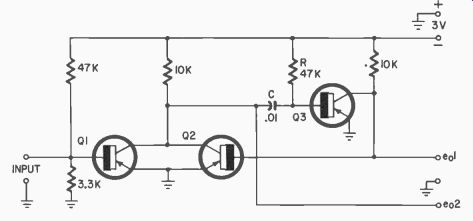
Fig. 403. Monostable multivibrator. Consider eo1 high amplitude and eo2 low amplitude. Input trigger reverses amplitudes of outputs, for time governed by R-C. Circuit then flips back to original condition.

This circuit can be used to pass on a constant pulse signal to following circuits, resetting itself each time after doing so. Since its time interval can be precisely set (by varying R-C ), a series of these circuits, (one energizing the other), can be used as a commutator suitable for decoding a train of pulses when the output of each is connected to one input of a coincidence circuit. Fig. 403 is another circuit for connecting transistors, this time three, in a multivibrator circuit. Fig. 404 shows typical waveforms.

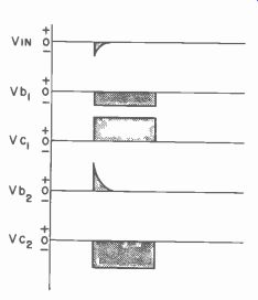
Fig. 404. Waveforms for monostable multivibrator.

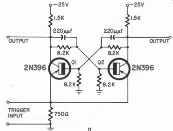
Fig. 405-a. Emitter input type bistable flip-flop multivibrator.

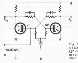
Fig. 405-b. Base input type bi stable multivibrator. Initially, Q2 conducts, QI does not. First negative pulse makes Q1 conduct. Remains so until positive pulse stops Q1

Basic bistable multivibrator circuits are shown in Figs. 405-a and b.

In these circuits, either transistor may start conducting first; which ever one does takes control and continues to conduct until an input pulse changes this state. The pulse required may be either positive or negative, depending upon where and when it is fed into the circuit.

If we assume that Q1 starts conducting first, then a positive-pulse input would stop Q1 and start Q2 conducting. Q2 would continue conducting until a negative-pulse input was received at the base of Q1 which would cut Q2 off and turn Q1 on. Thus, there are two stable states, and different input-pulse polarities are required to change them.

This binary (ON-OFF) circuit is also used in computers and counters.

It may be modified with diodes or other transistors to insure that the proper polarity input goes to the right transistor for switching, but basically they all operate in the same manner.

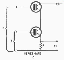
Fig. 406-a. In series gate, transistors are normally non-conducting. Simultaneous negative pulse at inputs A and B will drive transistors into conduction.

If our control intelligence is in the form of a series of pulses (a pulse train) we must have a means of separating these pulses and routing them independently to the various control circuits. This circuit can also be used as a form of pulse discriminator.

In addition to multivibrators, we can also use coincidence or gating circuits. Three basic forms of these electronic-controlled switches are given in Fig. 406.

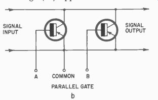
Fig. 406-b. In parallel gate, transistors conduct until a positive pulse is fed to the bases.

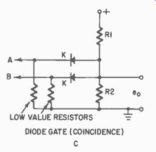
Fig. 406-c. Coincidence diode gate.

Normally, the diodes short-circuit R2.

If positive pulses are applied to A and B simultaneously, the diodes stop con ducting and voltage eo appears across R2.

Fig. 406-a shows the series gate. The two transistors are considered normally to be non-conducting and therefore there is no voltage developed across resistor R. To make both transistors conduct at the same time, a negative pulse must be received at the base of each (from inputs A and B) simultaneously. When these two pulses exist, then both transistors conduct and a voltage (eo) appears across R.

Diodes, too, can be used for gating purposes, as shown in Fig. 406-c.

In this case, two diodes are connected across R2, half a voltage divider consisting of R1 and R2. Each diode is connected and so biased that they conduct through a very low value resistor. Both effectively short circuit R2 and no output is obtained.

When positive pulses are fed to input terminals A and B, they bias the diodes and prevent conduction. This opens the short circuit across R2 and a voltage appears. Note, again, that both inputs A and B must be present simultaneously and be of the correct polarity to reverse bias the diodes.

Fundamental concepts of high speed pulse control

Now that we have some understanding of a few circuits that can be used, let us consider how we can use a transmitted series of ten pulses.

Nine of these pulses can be used for some control operation. For example, number 2 pulse will control the rudder, moving it to the right; number 3 will move the rudder to the left; number 4 will give up elevator; number 5 controls down elevator; number 6 increases motor speed; number 7 decreases motor speed, etc.

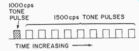
Fig. 407. A pulse "train" with "marker".

There is a reason we do not use number 1 to control a function.

Number 1 will be used to identify the pulse train itself. Refer to Fig. 407. We have specified that the first pulse will be a 1,000 cycle tone; all the other pulses will be 1,500 cycle tones.

There are other ways to identify a pulse train, such as having the first pulse wider than the rest; by sending two pulses with a very close spacing compared with the rest of the pulses, or by having the first pulse narrower than the rest. The circuitry to decode such a pulse train is complicated. With two tones we can use the regular types of bandpass filters to separate the pulses more economically.

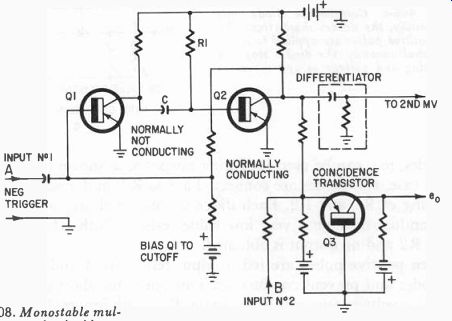
Fig. 408. Monostable multivibrator and coincidence circuit for series pulse decoding.

Fig. 408 is one circuit that can be used to decode a pulse sequence.

This is a monostable multivibrator, a differentiating circuit and a coincidence circuit. In the coincidence circuit the transistor (Q3) conducts until both inputs (one through Q1 and Q2) have a voltage of the proper polarity to offset the bias.

The circuit operates in this manner: First the 1,000 cycle tone pulse is separated from the others by a filter, as discussed earlier. This tone pulse is then passed through a diode rectifier connected so that the output pulse is negative with respect to ground. The pulse is then applied to input A. This causes Q1 to conduct, feeding the pulse to the base of Q2 through capacitor C. This, in turn, causes the collector voltage of Q2 to rise as Q2 is cut off. The voltage at the collector of Q2 is now more negative with respect to ground and a more negative voltage is now applied to one input of Q3. This voltage alone is not enough to cut off Q3.

If the second pulse of the train arrives, is separated, rectified negatively and applied to input B, while the negative voltage from the monostable multivibrator is applied to Q3, it will cause Q3 to stop conducting. The result is a negative pulse from the collector of Q3, since the voltage at the collector rises, or perhaps we should say, in creases negatively, since the p-n-p transistor requires a negative potential at its collector.

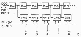
Fig. 409. Multivibrators and gates can separate control pulses.

The monostable multivibrator negative pulse to Q3 is also applied to the differentiating circuit where two sharp pulses (triggers) are produced. One is positive going and the other is negative going. The differentiator circuit now feeds a second monostable multivibrator and a second gating circuit and so on down the line for nine such circuits.

Fig. 409 is a block diagram of how the circuits are combined to make a decoder. (Fig. 410 shows how small the commercially manufactured multivibrators can be.) Note that there are nine outputs, one from each gating circuit. All the multivibrators are triggered by the single 1,000 cycle marker pulse, and as this is passed down the line, each gate is biased in turn, for its respective control pulse. When the last multivibrator is triggered, the action stops until another 1,000 cycle pulse starts the whole operation all over again.

Why do we use this? First, we could have an on-off type control.

For example, suppose we wanted to send only a signal for the left rudder. We would transmit only the 1,000 cycle tone pulse and the first 1,500 cycle control pulse. This code would be sent out over and over again as long as we wanted left rudder. When the pulse appears at number 2 terminal (Fig. 409) it will bias another transistor into conduction, controlling either a servo directly or a relay.

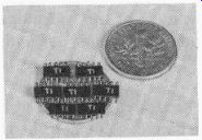
Fig. 410. Solid-state flip-flops make possible a pulse decoder [10 channels] smaller than a reed decoder. (Texas Instruments Co.)

Pulses 3 through 10 are not transmitted and we cannot send any more pulses until the same time interval has passed as would be required if all ten pulses had been sent. Thus we have to arrange, through a ground-control coder, that the pulses are transmitted automatically. In a mechanical method, a motor-driven arm can be rotated over ten contacts every revolution. The first contact would be connected to the 1,000-cycle oscillator and all other contacts to the 1,500-cycle oscillator. The arm, in turn, is connected to the transmitter modulator. As the arm rotates over these contacts, the transmitter sends out the 1,000 cycle tone pulse followed by nine 1,500 cycle tone pulses.

With control switches placed in series with each of the nine 1,500 cycle coder contacts (Fig. 411) only the closed switches will allow a pulse to be sent when the pickup arm is in that position. The coder motor speed must be adjusted so that it exactly matches the time interval required by the monostable multivibrators. In this way, each pulse arrives at its respective gate at the instant the gate is made conducting by its multivibrator.

Here is what we have gained by this method. First, if the pulse transmission rate is fast enough, the effect on the control equipment is as though they were all transmitted simultaneously. Second, there can be any combination of control functions without spillover from one channel into another. Third, control can be proportional in each channel provided the on-off control switches are replaced with another switch which would regulate whether a control pulse was sent every revolution of the motor, or once every two revolutions or once every three revolutions.

We can thus have a control system where the control deflection is proportional to the rate of pulse arrival. For example, if we send a ...

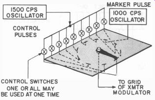
Fig. 411. A mechanical coder for pulse trains.

... right rudder pulse only once every five revolutions of the coder wiper arm, this would be a small rudder deflection, while if this pulse were sent every revolution this would be full rudder deflection. As to a method of arranging the coder circuit for a variable pulse transmission rate to occur, we leave that to your ingenuity.

Summarizing then, this system can offer simultaneous control over as many channels as the coder and decoder are built to handle. Each pulse would use the full transmitter modulation and thus arrive with maximum power for the maximum range and reliability. With the small-sized components now available for use with transistors and diodes, the decoding units can be made small, light and compact.

A pulse sorter using ferrites and transistors

We have examined one type of pulse decoder which might be suitable for simultaneous-proportional control, in which the proportional feature was obtained from how often the individual control pulses were transmitted. Now let us consider a pulse sorter that will not only separate the pulses but, in addition, will preserve the width of the control pulse. This makes it possible to use width variation to obtain proportional control.

With this system, the pulses as well as the spaces between them are in microseconds--truly a high speed system when compared to more common radio control methods. All other characteristics concerning the unlimited number of channels, etc., apply.

Before going into the circuit proper, we must understand the operation of an additional circuit element that is used, the ferrite core.

Refer to Fig. 412-a in which a linear core is shown with three windings. Also shown (in Fig. 412-b) is a magnetic core hysteresis curve.

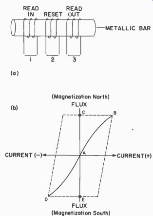
Fig. 412. Three-winding coil with ferrite core [a] and magnetic core hysteresis curve [b].

The core can be magnetized in either direction and, once magnetized in a given direction, will hold this magnetization until a reverse current flow reverses the magnetic polarity.

On the hysteresis loop, Fig. 412-b, point A represents the initial condition of the core, when it is not magnetized in either direction.

The curve A to B indicates that a current is flowing through, say, the read-in winding. Note that the flux reaches a maximum at point B.

The current then decreases to zero but the bar remains magnetized north (point C ). It remains in this condition although no current flows in any winding.

Suppose that some time later the reset winding is energized with a current which flows in a direction opposite to that of the first. Again, on the curve, as the current starts to build up (on the negative side of the current axis in Fig. 412-b), the flux first remains the same, then suddenly drops to point D. This drop means that the molecules in the core are now reversed. The end which was north is now south. Again the current decreases to zero and the bar is magnetized (E) in this new direction (south).

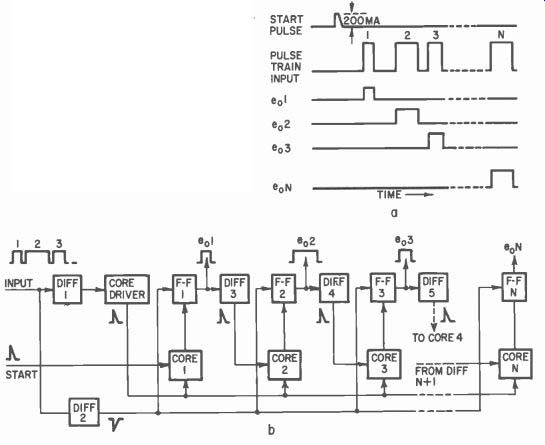
Fig. 413. Block diagram of pulse sorter. Width of each pulse [drawing a] sent into sorter is reproduced at outputs e. Last output eoN [drawing b] of sorter can be used to pulse core 1, thus setting up the sorter for the next pulse train. Differentiators 3, 4 and 5 set up cores for pulse from core driver. [Electronics Magazine.]

A meter placed across the read-out winding during this flux reversal would have given a quick jump of its pointer. If we send in another reset pulse, we will not get a read-out pulse because the core magnetism does not change. If, however, we feed in a read-in pulse, we do have a flux reversal and a read-out pulse is produced. We will get a positive-going pulse when, for example, we send a read-in pulse and a negative-going pulse when we send a reset pulse. The circuitry following such a core can use either one or the other or both of these output pulses, depending on the application. Although we have shown a bar or rod in this example, the core is normally circular, a donut or toroid which has a very high permeability and is capable of a large flux change in spite of its tiny size.

Fig. 413 is a block diagram of the ferrite core system. The start pulse sets the sorter to receive the pulse train, as in the previous decoder. This pulse switches ferrite core number I OFF, which turns off transistor flip flop ( another name for a multivibrator) number 1 ( F-Fl ). The leading edge of the first input pulse is shaped into a positive pulse by differentiator number 1 which then pulses the core driver.

The output of the core driver switches core number 1 ON which then feeds a positive pulse to flip flop number 1. Flip flop number 1 ( which sorts out the first pulse of the train ), is now pulsed into its ON condition.

The trailing edge of the first input pulse is shaped into a negative pulse by differentiator number 2 which is fed, in turn, to flip flop number 1. Flip flop number 1 then goes OFF and thus has duplicated the first pulse of the train.

When flip flop number 1 went ON, it fed a negative pulse to differentiator 3 setting up core 2 for the next input pulse of the train in the same way as the start-pulse prepared core 1 for the first input pulse. Flip flop number 2 and the following flip flops form symmetrical pulses from the following pulses at their outputs the same way that flip flop number 1 did.

Circuit details

In Fig. 414 Q1 and Q2 feed 200 ma pulses to the cores. For core read-in 2 ampere turns are required, and for a margin of safety, each core is wound with 12 turns. About 0.5 volt is produced by each turn of the output winding, and each flip flop transistor, such as Q3, requires a trigger pulse of 2 volts. For a safety margin, the core output winding has 5 turns. The reset winding, like the read-in, requires 2 ampere turns. It also has 12 turns.

The 200 ma reset pulses are produced by the flip flop output stages.

An output stage transistor with a nominal beta of 40 requires 5 ma for its base circuit from its flip flop to produce the 200 ma pulse. This is the reason for the large value of C1 .

The transistors such as Q2 and Q5 that drive cores are biased so that only the collector cutoff current, about 5 microamperes, flows between pulses. Thus the drivers appear as impedances of at least 1 megohm.

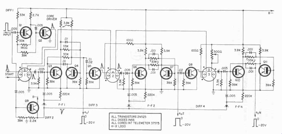
Fig. 414. Circuit of pulse sorter. [Electronics Magazine]

The flip flops are turned off and on by positive and negative triggers, respectively. Positive triggers have low amplitudes. Negative triggers turn on the flip flops when the pulse level rises above a well defined threshold level. These negative trigger pulses are supplied by Q9. Each flip flop delivers a positive going pulse for an output.

Cores can be scramble wound with No. 28 or 30 Formex wire. The windings are all in the same direction, and concentrated in three areas of the core. These cores do not function reliably above 60° Centigrade (about 140° Fahrenheit.) Pulse discriminator for proportional control We have covered some ways of separating the pulses in a pulse train and we have given a circuit which will preserve the input pulse widths. It was suggested that we could use this width variation for proportional control of each channel. Now we want to consider a possible method of doing so.

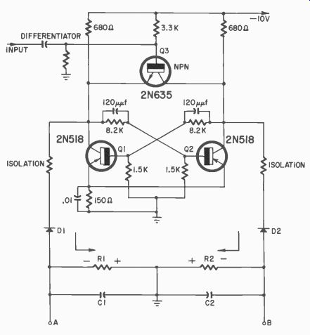
Fig. 415. Pulse discriminator and multivibrator.

Fig. 415 is a conventional bistable or flip flop multivibrator schematic with two circuit additions. The first is transistor Q3, an n-p-n type which is connected in a manner that will insure a positive input pulse will trigger the circuit in one direction and that a negative pulse will trigger it in the reverse direction. Added components are the two diodes, D1 and D2, R1 and R2, and C1 and C2.

For the theory of operation, assume that its input is the output of Fig. 414. Let this square wave output be eo1:

If this particular channel has a symmetrical output pulse (a pulse whose spacing is equal to its width) and if it feeds the differentiator shown in Fig. 415, it would have the waveforms shown in Fig. 416.

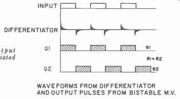
Fig. 416. Symmetrical output pulses and their differentiated waveforms. WAVEFORMS FROM DIFFERENTIATOR AND OUTPUT PULSES FROM BISTABLE M.V.

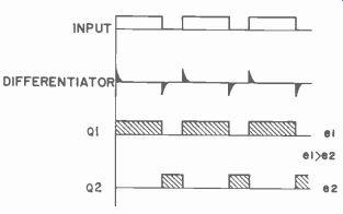
Fig. 417. Effect of pulse width wider than spacing.

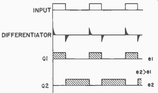
Fig. 418. Effect of spacing wider than pulse width.

The positive differentiated spike turns on Q1 while the negative spike turns on Q2. Since the pulse widths and spacings are equal, each transistor (Q1 and Q2) are on the same amount of time.

Whenever Q1 flow through D1 to R1-C1, as indicated by the arrow. The same would be true for Q2. Now, since the pulse widths and spacings are equal, the currents through R1-R2 are equal but in the opposite direction, thus the output across A and B is zero. Capacitors C1 and C2 are needed to store the voltage drops momentarily during the time when the collector voltages drop. Two isolation resistors are used to prevent any possible interaction between the R-C filters and the multivibrator time constant components.

The input pulse width in Fig. 417 has increased and the spacing decreased. The differentiated spikes are no longer symmetrical. Q1 remains cut off longer than Q2. Therefore the voltage delivered to R2-C2 is longer and thus becomes higher in amplitude than that from Q 1 . This unbalances the output and point if in Fig. 415 will be positive with respect to point B. The actual voltage produced would be proportional to the pulse width unbalance.

Fig. 418 shows the reverse situation, where the input pulse width is narrower than the spacing. This unbalance is in the opposite direction and point A becomes negative with respect to point B. Again the actual voltage produced would be proportional to the unbalance in pulse width and spacing.

By varying the pulse width and spacing in a train of ten pulses, we can command a change of direction by a change of voltage polarity, and the degree of change by the amount of either the positive or negative voltage.

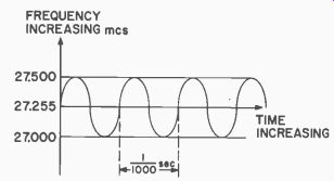
Fig. 419. The frequency-modulation concept.

Simultaneous transmission of pulse rates Another method of obtaining proportional control through pulses is to transmit several pulse rates simultaneously. If we were to have four tones, and each capable of being pulsed at a varying rate (spacing and width constant), we would have the basis for proportional and simultaneous control over four functions. This would mean there would have to be four bandpass filters to separate the four channels.

We will have to transmit four tones simultaneously, however. This will mean a little more amplification after each filter to get sufficient tone strength. The rates can then be averaged in a simple diode counting circuit which would produce a voltage proportional to the pulse rate to serve as a basis for proportional control of many functions.

Frequency modulation of a pulse repetition rate

Another possibility is that of using frequency modulation techniques combined with pulses to achieve control. This idea would help maintain the strong modulation characteristics we desire.

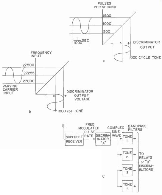
Fig. 420. The FM pulse concept [a], FM receiver operation [6] and block diagram of system decoding frequency-modulated pulse-rate code [c]. Discriminator A is an audio type circuit designed to have zero output when pulse resting frequency is received. B discriminator is similar to A except that it is designed for individual tone frequencies.

Review, for a moment, the concept of frequency modulation. When we frequency modulate a carrier, we make the carrier go higher, then lower, than the resting (center) frequency at the desired tone rate.

Fig. 419 shows this concept as applied to a 27.255 mhz rest frequency when modulated with a 1,000 cycle tone. Note that the carrier is changed by the 1,000 cycle sine wave in a sinusoidal manner from 27.255 to 27.500 back to 27.255, down to 27.000 and back to 27.255 mhz at a. 1,000 times per second rate.

What the FM receiver does when it picks up this varying wave is shown in Figs. 420-a,-b. Note that the varying carrier goes in, on the left, and comes out on the bottom as a 1,000 cycle per second positive and negative voltage variation. This voltage variation is the modulation tone at the transmitter.

We cannot frequency modulate the carrier on any of the radio control frequencies which the FCC has allocated for radio control since these are spot frequencies. We can, however, utilize this principle by frequency modulating a pulse rate to obtain simultaneous trans mission of many control signals. The possible receiver action is indicated in Fig. 420-c. Note that we would apply the pulses to a tone type frequency discriminator and as an output get the tone causing the rate variation.

It is interesting to note that when transmitting pulses (if the pulses are applied to a transformer or to an R-C network) we can recover a cycle for each pulse. In this case then, the frequency modulated pulses, when applied to a discriminator, would produce an output tone which would be exactly identical with the tone causing the pulse frequency modulation.

If we were to modulate these pulses with a combination of four different tones, we would recover a complex wave with a pulse discriminator. This wave could then be broken down and the individual tones separated by bandpass filters.

Two useful pulse shapers

Two simple pulse shaping circuits are given in Figs. 421 and 422.

In Fig. 421 an input drives the transistor to saturation and to cut off.

This could be a trigger type input. Capacitor C is charged rapidly through D1 and discharges slowly through D2 into load R. Thus a square wave is produced from a trigger input.

In Fig. 422, a sine wave is rectified by diode D1 and applied, in the correct polarity, to the n-p-n transistor Q1. The output of Q1 is amplified by Q2 which is driven to saturation and cut off to produce the square wave pulses shown. If the sine wave input to D1 were to constantly change slightly in frequency, the pulse output of Q2 would be pulses frequency modulated, in a like manner.

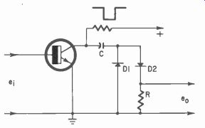
Fig. 421. Pulse shaping circuit. This circuit produces square waves.

Mechanical decoder pulse control system

Decoders for pulse command work seem limited only by the imagination and the mechanical and electronic systems used. This mechanical decoding and control system was developed to obtain control over the rudder (proportional steering), the elevator (trim) and the motor of a model aircraft engine. The system uses but one channel with the pulse-width--pulse-spacing variation type of command-code modulation.

The concept of rudder steering used in this code is well known, and it will be assumed that the reader understands this method of control.

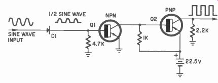
Fig. 422. Pulses produced from sine wave [tone].

The elevator operating code derived from this is: Carrier on solid, no pulsing equals up-trim; carrier off, no signal, equals down-trim. The engine control 'circuit code is a mixture of a full-on command, followed immediately by a full-off command, after which pulsing may be resumed. A fail safe provision is provided by mechanical elevator stops which prevent the model from going into a dive in case of loss of signal.

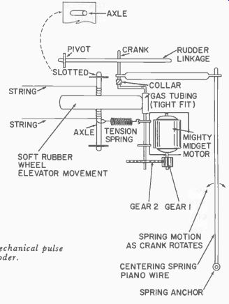
Fig. 423. A mechanical pulse decoder.

The basic system is shown in Fig. 423 and is constructed around a single Mighty Midget motor and its integral gearing and gear shaft.

Note that in this drawing, which illustrates the rudder and elevator control mechanisms, the large gear shaft has been bent into a crank, and that there is a piece of aluminum tubing connected to the crank by one flattened end and to a piano wire spring at the other. The spring and the tubing center the rudder. A piece of gas-line tubing has been placed on the gear shaft so that it provides a friction drive for the soft rubber elevator-movement wheel. Note also that the elevator-movement wheel axle is set at the bottom into a good tight bearing fit, while at the top, the axle is slotted so that it can be pulled to the left far enough so it will not touch the gas-line tubing on the gear shaft. Next locate the tension spring just below the elevator-movement wheel; this spring normally holds the wheel against the gas-line tubing so that a good friction drive is produced.

Fig. 424 shows how the rudder is connected through strings to the steering-control mechanism. The circle indicates the path of the tip of the rudder crank if it were to rotate freely. The dotted linkage is the centering tubing described previously. Fig. 424-a shows the rudder linkage in the neutral position. The crank will oscillate back and forth from this neutral position when equal width pulses and spaces are received. In Fig. 424-b the rudder crank is displaced from center by a code of unequal width pulses and spaces; the rudder-linkage bar is moved as shown, and the rudder is deflected.

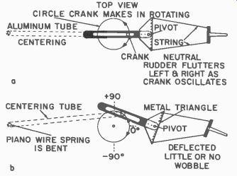
Fig. 424. Rudder is connected by strings to steering-control mechanism. Crank must be able to rotate. Must also have some spring tension at neutral.

In most applications for this type of pulse control, a centering spring is connected to the crank itself and pulls the crank back to neutral. In this case, the maximum restoring force occurs at somewhat less than 90° crank displacement, when the line of action is perpendicular to the crank position. With the spring arrangement shown, with the force ahead of the crank, the maximum torque will not occur until somewhat after the 90° crank position and thus the system is more linear near the ends of the swing. This means a larger deflection of the rudder is possible under normal operating conditions. Because of the slotted bar the crank can oscillate at the extreme positions and will not impart any motion ( wobble) to the rudder itself. Actually the wobble gets smaller as the crank moves further from neutral.

As long as only a rudder-control operation is desired, the crank oscillates between the plus 90° and minus 90° positions. It does not turn through a revolution. But suppose we want to change the elevator trim.

If we hold the signal ON the crank will now rotate. The rudder will wobble, but its dwell time on each side of center will be the same so there is no change in model direction. What does happen, however, is that the rubber wheel (Fig. 423) which is now touching the gas-line tubing is turned. The elevator, connected to the axle of the rubber wheel through two lengths of string or cord, is moved into a new position as the string on one side of the rubber wheel tightens and that on the opposite side loosens by the same amount. As soon as the desired elevator trim is achieved, the constant signal is stopped and the pulse signal resumes, and the control crank returns to oscillate about its neutral position. Note that to change the elevator trim in the opposite direction we would merely cut off the signal until the desired trim was obtained and then resume pulsing again.

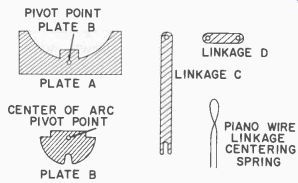
Fig. 425. Parts required for mo tor control. Use thin aluminum pieces.

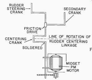
Fig. 426. Details of secondary crank addition.

Now here's the reason for the slotted bearing at one end of the elevator wheel axle. Since we have provided physical stops to prevent the control surface from moving too far from neutral, we must also have some means of stopping the rubber wheel to prevent breaking the string, or at least smoothing the friction surface. Note, then, how the elevator wheel motion is stopped when the limit is reached. The string on the one side will continue to tighten. As it does so, it pulls the elevator-wheel axle which slides in its top bearing slot away from the gas-line tubing. A continued signal for still more elevator deflection will have no effect. Now, if we want to reverse the crank direction to return the elevator to its original position the tension spring will pull the elevator wheel shaft tight against the gas-line tubing so that the friction drive is re-established.

Since the elevator wheel is large compared to its axle, a very gradual control of the elevator is possible. One revolution of the axle will wind up only a very small amount of string. By changing the diameter of the wheel and the axle roller, the speed of elevator movement can be changed.

The final portion of the mechanism is a little more complicated.

First, examine Fig. 425 which shows the parts required. These five parts are not to scale and must be custom made for each system. Now examine Fig. 426 which shows modifications to the gear shaft. A U-section is added as shown, and a second crank (secondary crank) is added. This secondary crank is so connected to the gear shaft that it is tight enough to hold a position while the gear shaft rotates when desired.

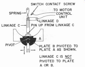
Fig. 427. Assembly of switch parts.

Next refer to Fig. 427 which shows how the five parts of Fig. 425 are assembled. Plate B is pivoted to plate A and is free to rock back and forth. Linkage C is positioned so that its pivot to linkage D is directly above the pivot connecting A and B. Linkage D is then pivoted at its other end to a base plate. The spring is adjusted so that it will hold linkage C in the position shown and keep the pin in linkage C against the center square of plate A as shown. Linkage C should move easily left or right under plate A or up and down as shown by the arrows at the lower end of Fig. 427. The anchor pivot for D should be tight enough so that both linkages do not have any end play, yet is free enough to allow easy pivoting.

The same arrangement is shown in Fig. 428, and a circle indicating the rotary motion of the rudder steering crank has been added. Note that the secondary crank is inserted in the slot of plate B. When the rudder crank is in the neutral position, it is exactly opposite the slot in plate B.

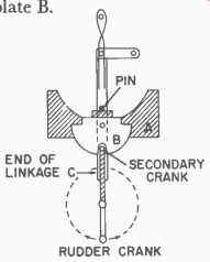
Fig. 428. Position of primary and secondary cranks in normal operation.

Fig. 429 is a simplified side view of the mechanism assembled with the other components. The only change is that linkage C is placed above plates A and B, and its pin goes down as shown.

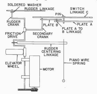
Fig. 429. Side view details of mounting. Rudder crank engages end of link age A during rotation.

Now see Fig. 430 for the operation. With the secondary crank inserted in the slot of plate B and the rudder crank exactly opposite ( Fig. 430-a ), we start the system by sending control pulses. The rudder crank can move back and forth as required for steering and plate B will oscillate back and forth also. Steering is perfectly normal.

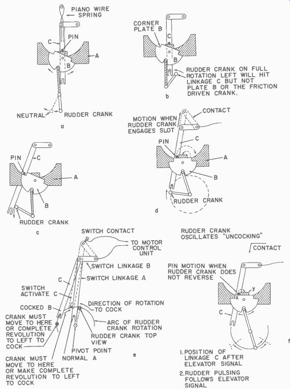
Fig. 430. Plate B oscillates [drawing a] as rudder crank oscillates. Linkage C remains in position shown. Plate B [drawing b] is restricted from moving further by mechanical stop. Friction drive to secondary crank allows it to stop while motor keeps turning rudder crank. Rudder crank [drawing c] moves linkage A so pin drops into B-plate indent "cocked position". Note that pin will move to the right after crank passes so slot in A will rest on crank circle. If rudder crank [drawing d] immediately reverses, it engages slot, pushing C up as it goes "firing" [linkage C touches contact]. Drawing e shows the movement of linkage C. When plate B oscillates [drawing f] as the rudder oscillates, shoulder X rises to move pin to Y. Linkage A does not move back to take contact.

In Fig. 430-b an ON signal starts the rudder crank motion. Plate B is pushed to the left until its corner rises level with the square midsection of plate A. It is held there by means of a mechanical pin stop ( which, for simplicity, we have not shown ).

Remember that the crank which moves this plate is friction connected in the gear axle. The rudder crank then continues to rotate as shown in Fig. 430-c and as it does so, it hits linkage C and moves it over until its pin drops in the corner of plate B. The spring pushing down locks it in this position. The rudder crank keeps going but linkage C now remains in this deflected position. Note that after the rudder crank passes linkage C in its locking-in position, the linkage settles so that its slot is directly in line with the rudder crank circle of rotation. If we now send an off signal and hold this momentarily, the rudder crank reverses its rotation (Fig. 430-d) . As it does so, the rudder crank moves into the slot at the end of linkage C and forces it back and up until it closes the contact placed as shown in Figs. 430-e and f ( an adjustable screw contact is shown; this could be a spring type contact so it can bend) . As the rudder crank continues its rotation, linkage C is moved over to the right position where it slides down the circle of plate A to come to rest against the square center of plate B which has also moved to the right. It will remain there even though the rudder crank continues to rotate for a second or so longer.

Now assume that we resume sending the pulse signal. Immediately plate B starts to oscillate and as it swings to the right, its corner pushes the pin on linkage C, moving it up high enough to slide onto the square center section of plate A. Due to the spring tension the linkages return to their neutral positions and everything is back to normal again.

If an elevator signal is now transmitted the contact will not be closed unless we send an up elevator signal and follow it immediately with a down elevator signal. If pulsing starts, even for a second, be tween up and down elevator signals, the motor control contact mechanism will un-cock and will not make connection to the motor control unit.

We can send elevator signals, then, without this part of the unit being affected. Should we send an engine speed-change signal (and remember, this must be an ON signal followed immediately by an OFF signal), the elevator is hardly affected since the length of time required to cause the engine change is extremely short. Actually, we only require one revolution of the rudder crank in one direction and then an immediate reverse back to neutral. The elevator control string won't wind since the two rotations are equal.